Winter Olympics Medal Analysis

Author

Octavia Steiger

Published

April 6, 2026

Why does Norway win so much?

Norway has a population of just 5 million people, yet it sits at the top of the all-time Winter Olympic medal table with 318 medals, more than 40 ahead of the United States despite the US having around 60 times the population. So what’s going on?

To find out, I looked at data from every Winter Olympic Games since Chamonix 1924, testing three possible explanations: wealth, population size and home advantage. The short answer: all three matter just not equally.

Before diving into the results, it helps to understand exactly what data sits behind this analysis and how it was built.

The pipeline: scrape –> clean –> merge with World Bank data –> analyse –> visualise

1. The data

I used two main datasets for this, one tracking Olympic medal outcomes going back a century, and one capturing the economic context behind each competing nation.

Olympic Medals (Olympedia):

Scraped from Olympedia, covering all 24 Winter Games from Chamonix 1924 to Beijing 2022. Each row represents one country’s performance in a single Games (1,163 country-year observations in total).

Variable	Description
`NOC`	National Olympic Committee country code
`Year`	Olympic Year (1924 - 2022)
`Gold / Silver / Bronze`	Medal counts for that Games
`Total`	Sum of all medals won
`Host`	1 if the country hosted that year, 0 otherwise

Economic Indicators (World Bank):

GDP per capita (Current USD, indicator NY.GDP.PCAP.CD) and population (SP.POP.TOTL) fetched via the World Bank API, then matched to each country-year in the medals dataset.

A note on tied medals: In 27 events where multiple athletes tied for the same medal position, each tied nation received full medal credit, consistent with how the IOC handles ties in official records.

2. Building the dataset

2.1 Collecting the Medal Data

Official Olympic data was not available as a download, so the data had to be scraped directly from Olympedia (https://www.olympedia.org).

I built a web scraper (scrape.py) that fetched the medal table for each of the 24 Winter Olympic Games. Each page returned an HTML table listing every event alongside gold, silver and bronze medalists and their countries.

The raw data came back wide, with separate columns per medal, country names in inconsistent formats, sports category headings mixed into the results rows and combined NOC codes where medals were tied.

Not all NOCs appear in each Games, the number of competing nations has grown over time, from around 19 nations in 1924 to over 90 today.

Show code

import pandas as pd
medals = pd.read_csv('../data/clean/medals_clean.csv')
print(f"{len(medals)} events scraped across {medals['year'].nunique()} Games")
medals.head(10)

1163 events scraped across 24 Games

	year	sport	event	gold_name	gold_noc	tie_gold	silver_name	silver_noc	tie_silver	bronze_name	bronze_noc	tie_bronze
0	1924	Alpinism	Alpinism, Open	Mixed team	MIX	False	—	—	False	—	—	False
1	1924	Bobsleigh	Four, Men	Switzerland 1	SUI	False	Great Britain 1	GBR	False	Belgium 1	BEL	False
2	1924	Cross Country Skiing	18 kilometres, Men	Thorleif Haug	NOR	False	Johan Grøttumsbraaten	NOR	False	Tapani Niku	FIN	False
3	1924	Cross Country Skiing	50 kilometres, Men	Thorleif Haug	NOR	False	Thoralf Strømstad	NOR	False	Johan Grøttumsbraaten	NOR	False
4	1924	Curling	Team, Men	Great Britain	GBR	False	Sweden	SWE	False	France	FRA	False
5	1924	Figure Skating	Singles, Men	Gillis Grafström	SWE	False	Willy Böckl	AUT	False	Georges Gautschi	SUI	False
6	1924	Figure Skating	Singles, Women	Herma Planck-Szabo	AUT	False	Beatrix Loughran	USA	False	Ethel Muckelt	GBR	False
7	1924	Figure Skating	Pairs, Mixed	Austria	AUT	False	Finland	FIN	False	France 1	FRA	False
8	1924	Ice Hockey	Ice Hockey, Men	Canada	CAN	False	United States	USA	False	Great Britain	GBR	False
9	1924	Military Ski Patrol	Military Ski Patrol, Men	Switzerland	SUI	False	Finland	FIN	False	France	FRA	False

2.2 Cleaning the Data

Sorting out the sport categories

The scraped HTML table included two types of rows: actual event results and section headings that just said the sport name. These headings were not real results, they had no medalists data or NOC codes, however they did have the sport name of each event which is information I still needed.

In clean.py, I identified the heading rows (any row where all medal columns were empty), extracted the sport name, forward filled it down to all the event rows below, then dropped the headings.

Show code

print("Sports present in the dataset:")
print(sorted(medals['sport'].dropna().unique().tolist()))

Sports present in the dataset:
['Alpine Skiing', 'Alpinism', 'Biathlon', 'Bobsleigh', 'Cross Country Skiing', 'Curling', 'Figure Skating', 'Freestyle Skiing', 'Ice Hockey', 'Luge', 'Military Ski Patrol', 'Nordic Combined', 'Short Track Speed Skating', 'Skeleton', 'Ski Jumping', 'Snowboarding', 'Speed Skating']

Dealing with tied medals

Occasionally there were two countries that shared a podium position, for example two gold medalists and no silver. In the raw data these appear as a single combined entry in the NOC column rather than as two seperate rows.

These needed to be detected and split into two rows, otherwise any country-level analysis would be inaccurate. Within the cleaning step these are flagged using the tie columns and then are split into seperate rows in a later step in the pipeline, so that both countries get the credit for the medal in the analysis.

Show code

tied = medals[medals['tie_gold'] | medals['tie_silver'] | medals['tie_bronze']]
print(f"Events with at least one tied medal: {len(tied)}")
tied[['year', 'sport', 'event', 'tie_gold', 'tie_silver', 'tie_bronze']].head(8)

Events with at least one tied medal: 27

	year	sport	event	tie_gold	tie_silver	tie_bronze
12	1924	Speed Skating	500 metres, Men	False	False	True
27	1928	Speed Skating	500 metres, Men	True	False	False
61	1948	Alpine Skiing	Downhill, Men	False	False	True
101	1952	Speed Skating	500 metres, Men	False	False	True
126	1956	Speed Skating	1,500 metres, Men	True	False	False
149	1960	Speed Skating	1,500 metres, Men	True	False	False
160	1964	Alpine Skiing	Giant Slalom, Women	False	True	False
174	1964	Figure Skating	Pairs, Mixed	False	True	False

There are relatively few, but they matter. :::{.callout-tip} ## Why this matters Ignoring ties would undercount medals for countries involved. Splitting them into seperate rows ensures every nation gets full credit which is consistent with how the IOC handles ties in official records. :::

2.3 Adding Economic Context

To test whether wealth or population drives success, each medal row needed to be merged with GDP and population data for the corresponding year.

Why I used the World Bank API

I needed two indicators for each country and year: GDP per capita and population size. Both indicators were fetched from the World Bank API (https://data.worldbank.org/) using the wbgapi package, which gave clean, standardised data without additional formating work.

The NOC to ISC problem

There was however a problem with merging the medal data with the World Bank data, as the medal data uses NOC codes to identify countries, whereas the World Bank data uses ISO country codes. This required a lookup table mapping each NOC to its closest modern equivalent, since some NOCs no longer exist or have since split into multiple countries.

The trickiest cases were the Soviet Union (URS), East Germany (GDR) and Yugoslavia (YUG) which are all heavy medal winners that no longer exist. For these I mapped to their largest successor state (Russia, Germany and Serbia) where economic data was available and excluded rows where I could not make a reasonable match.

Merging the datasets

Once both datasets used the same country codes, they were joined on country and year, giving a single dataset with two additional columns:

is_host : a flag marking whether the winning country was hosting the games that year, to test the impact of home advantage
log_gdp_per_capita and log_population: I took the log of both to account for diminishing returns, the gap between a poor and a morderately wealthy country matters more than the same gap at the top end of the scale.

Show code

final = pd.read_csv("../data/clean/worldbank_final.csv")
print(f"Final merged dataset: {len(final)} medal rows")
final.head(8)

Final merged dataset: 3493 medal rows

	year	event	noc	medal	iso_code	gdp_per_capita	population	host_noc	log_gdp_per_capita	log_population
0	1924	Singles, Women	AUT	gold	AUT	NaN	NaN	FRA	NaN	NaN
1	1924	Pairs, Mixed	AUT	gold	AUT	NaN	NaN	FRA	NaN	NaN
2	1924	Singles, Men	AUT	silver	AUT	NaN	NaN	FRA	NaN	NaN
3	1924	Four, Men	BEL	bronze	BEL	NaN	NaN	FRA	NaN	NaN
4	1924	Ice Hockey, Men	CAN	gold	CAN	NaN	NaN	FRA	NaN	NaN
5	1924	18 kilometres, Men	FIN	bronze	FIN	NaN	NaN	FRA	NaN	NaN
6	1924	Allround, Men	FIN	bronze	FIN	NaN	NaN	FRA	NaN	NaN
7	1924	500 metres, Men	FIN	bronze	FIN	NaN	NaN	FRA	NaN	NaN

Show code

missing = final['gdp_per_capita'].isna().sum()
total = len(final)
print(f'Rows with missing GDP per capita: {missing} ({100 * missing / total:.1f}%)')
print('These are mostly historic NOCs')

Rows with missing GDP per capita: 567 (16.2%)
These are mostly historic NOCs

The missing GDP rows are expected and unavoidable, as many of the older NOCs no longer exist and therefore do not have corresponding economic data in the World Bank dataset. Therefore, I excluded these rows from the regression but kept in the raw medal count so the all-time table remains accurate.

Data limitation

Around 16% of medal rows are missing GDP data, mostly from historical NOCs that no longer exist (URS, GDR, YUG). These are excluded from the regression but kept in the all-time medal counts so historical totals remain accurate.

3. A century of dominance

Show code

import matplotlib.pyplot as plt
import seaborn as sns

sns.set_theme(style='whitegrid', font_scale=1.1)
GOLD   = "#FFD700"
SILVER = "#C0C0C0"
BRONZE = "#CD7F32"
BLUE   = "#1f77b4"
alltime = pd.read_csv("../data/clean/alltime_table.csv")
cy      = pd.read_csv("../data/clean/medals_country_year.csv")
reg     = pd.read_csv("../outputs/regression_results.csv")
final   = pd.read_csv("../data/clean/worldbank_final.csv")

NOC_NAMES = {
    'NOR': 'Norway',    'USA': 'United States', 'AUT': 'Austria',
    'GER': 'Germany',   'FIN': 'Finland',       'SWE': 'Sweden',
    'SUI': 'Switzerland','RUS': 'Russia',        'CAN': 'Canada',
    'ITA': 'Italy',     'FRA': 'France',         'NED': 'Netherlands',
    'GDR': 'East Germany','URS': 'Soviet Union', 'TCH': 'Czechoslovakia',
    'EUN': 'Unified Team','JPN': 'Japan',        'KOR': 'South Korea',
    'CZE': 'Czech Republic','POL': 'Poland',     'GBR': 'Great Britain',
    'BEL': 'Belgium',   'YUG': 'Yugoslavia',    'LIE': 'Liechtenstein',
}

The table below shows the 15 most decorated nations, ranked by total medals.

Show code

import pandas as pd
summary = pd.read_csv('../outputs/summary_stats.csv', index_col=0)
summary.style.set_caption('Table 1: Top 15 nations by total Winter Olympic Medals')

Table 1: Table 1: Top 15 nations by total Winter Olympic Medals

	Avg Medals/games	Total medals	Games Attended
noc
NOR	18.700000	318	17
USA	16.200000	275	17
GER	24.400000	268	11
AUT	12.400000	211	17
CAN	12.200000	207	17
NED	9.000000	144	16
SUI	8.900000	142	16
SWE	8.000000	136	17
ITA	7.900000	135	17
FIN	7.600000	129	17
FRA	7.400000	126	17
RUS	19.700000	118	6
GDR	18.300000	110	6
KOR	8.800000	79	9
CHN	8.600000	77	9

Norway and the United States lead on total medals, both attending all 17 Games in the dataset. However, the average medals per Games column tells a more interesting story, by sorting by average medals rather than totals it reshuffles the rankings considerably.

Germany and the Cold War nations

Germany’s average of 24.4 medals per Games is the highest in the table desipte having only 11 appearances. This highlights how dominant West Germany and later reunified Germany have been when they competed. Russia (6 Games, 19.7 avg) and East Germany (6 Games, 18.3 avg) show even higher rates, however both stop competing after the Soviet era ended.

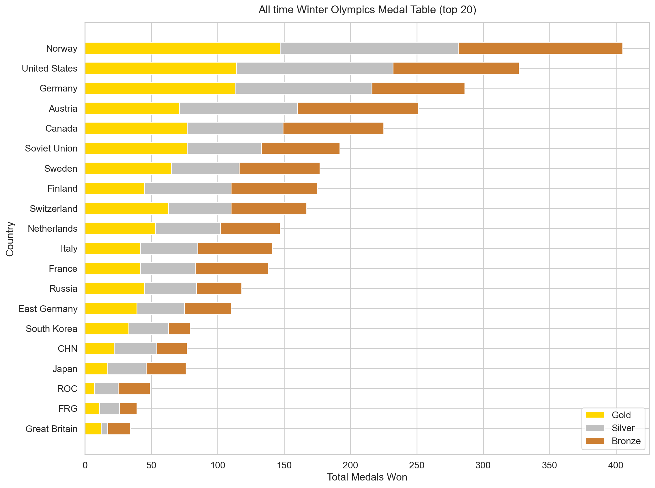
The chart below shows cumulative medals since 1924 across the top 20 nations. Norway’s bar is noteably gold, showing it doesn’t just compete but consistently wins. The US and Germany follow, both benefiting from size and long-term investment in winter sport.

Show code

alltime['country'] = alltime['noc'].map(NOC_NAMES).fillna(alltime['noc'])
fig, ax = plt.subplots(figsize=(12, 9))

ax.barh(alltime['country'], alltime['gold_medals'], label='Gold', color=GOLD, height=0.6)
ax.barh(alltime['country'], alltime['silver_medals'], label='Silver', color=SILVER, height=0.6, left=alltime['gold_medals'])
ax.barh(alltime['country'], alltime['bronze_medals'], label='Bronze', color=BRONZE, height=0.6, left=alltime['gold_medals'] + alltime['silver_medals'])

ax.invert_yaxis()
ax.set_title("All time Winter Olympics Medal Table (top 20)", fontsize=14, pad=12)
ax.set_xlabel("Total Medals Won")
ax.set_ylabel("Country")
ax.legend(loc='lower right')
fig.tight_layout()
plt.show()

Figure 1: Figure 1: Cumulative Winter Olympic medals for the top 20 nations since 1924. Norway’s gold-heavy bar reflects not just volume but consistent dominance across disciplines.

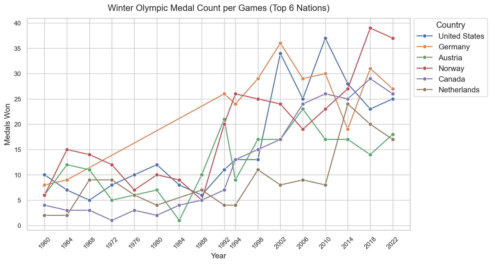
The all-time totals hides a lot of movement, so this chart tracks medals per Games for the top 6 nations.

Show code

top6   = cy.groupby('noc')['total_medals'].sum().nlargest(6).index.tolist()
subset = cy[cy['noc'].isin(top6)].copy()
subset['country'] = subset['noc'].map(NOC_NAMES).fillna(subset['noc'])

fig, ax = plt.subplots(figsize=(11, 6))
sns.lineplot(data=subset, x='year', y='total_medals', hue='country', marker='o', ax=ax)

ax.set_title('Winter Olympic Medal Count per Games (Top 6 Nations)', fontsize=14, pad=12)
ax.set_xlabel('Year', fontsize=12)
ax.set_ylabel('Medals Won', fontsize=12)
ax.tick_params(axis='both', labelsize=10)

ax.legend(title='Country', bbox_to_anchor=(1.01, 1), loc='upper left', borderaxespad=0.)

ax.set_xticks(sorted(cy['year'].unique()))
ax.tick_params(axis='x', rotation=45)
fig.tight_layout()
plt.show()

Figure 2: Figure 2: Medals won per Games for the top 6 nations by all-time count. The gap between 1936 and 1948 reflects the cancellation of the 1940 and 1944 Games due to World War II. You’ll also notice a clear spike for the United States in 2002, which lines up with the Salt Lake City Games being held on home soil.

Norway is consistently near the top throughout, with very few poor Games. Russia (URS before 1992) came on strong from the mid-1950s and dominated throughout the 1980s but then dropped off sharply after the Soviet Union dissolved. The dominance of wealthy nations raises the obvious next question: Is it just money?

4. Does money buy medals?

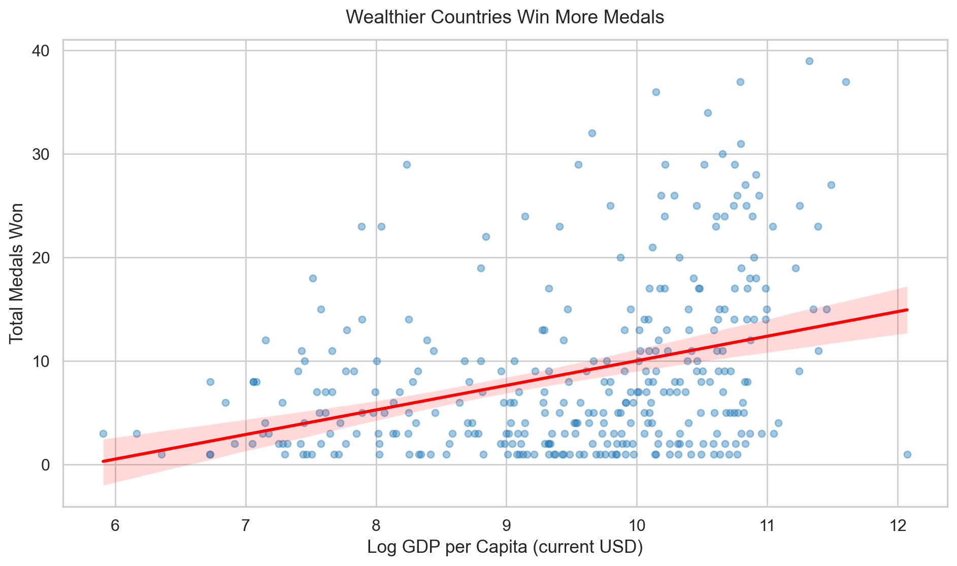
The scatter plot below plots log GDP per capita against total medals. The upward trend is clear, wealthier countries tend to invest more in training and facilities and it shows.

Wealth isn’t everything

Qatar and Singapore rank among the world’s wealthiest nations but have never won a Winter Olympic medal, so climate and sporting culture clearly matter alongside money.

Show code

plot_data = cy.dropna(subset=['log_gdp_per_capita', 'total_medals'])
fig, ax = plt.subplots(figsize=(10, 6))
sns.regplot(data=plot_data, x='log_gdp_per_capita', y='total_medals',
            scatter_kws={'alpha': 0.4, 's': 25, 'color': BLUE},
            line_kws={'color': 'red'}, ax=ax)
ax.set_title("Wealthier Countries Win More Medals", fontsize=14, pad=12)
ax.set_xlabel("Log GDP per Capita (current USD)")
ax.set_ylabel("Total Medals Won")
fig.tight_layout()
plt.show()

Figure 3: Figure 3: Relationship between log GDP per capita and total medals won across all country-year observations. The overall upward trend makes it clear that richer countries tend to win more medals. That said, the spread of points around the line is a reminder that wealth isn’t the whole story, other factors still matter.

Wealth clearly plays a role but there is one advantage no investment can buy and that is competing on home soil.

5. The home advantage

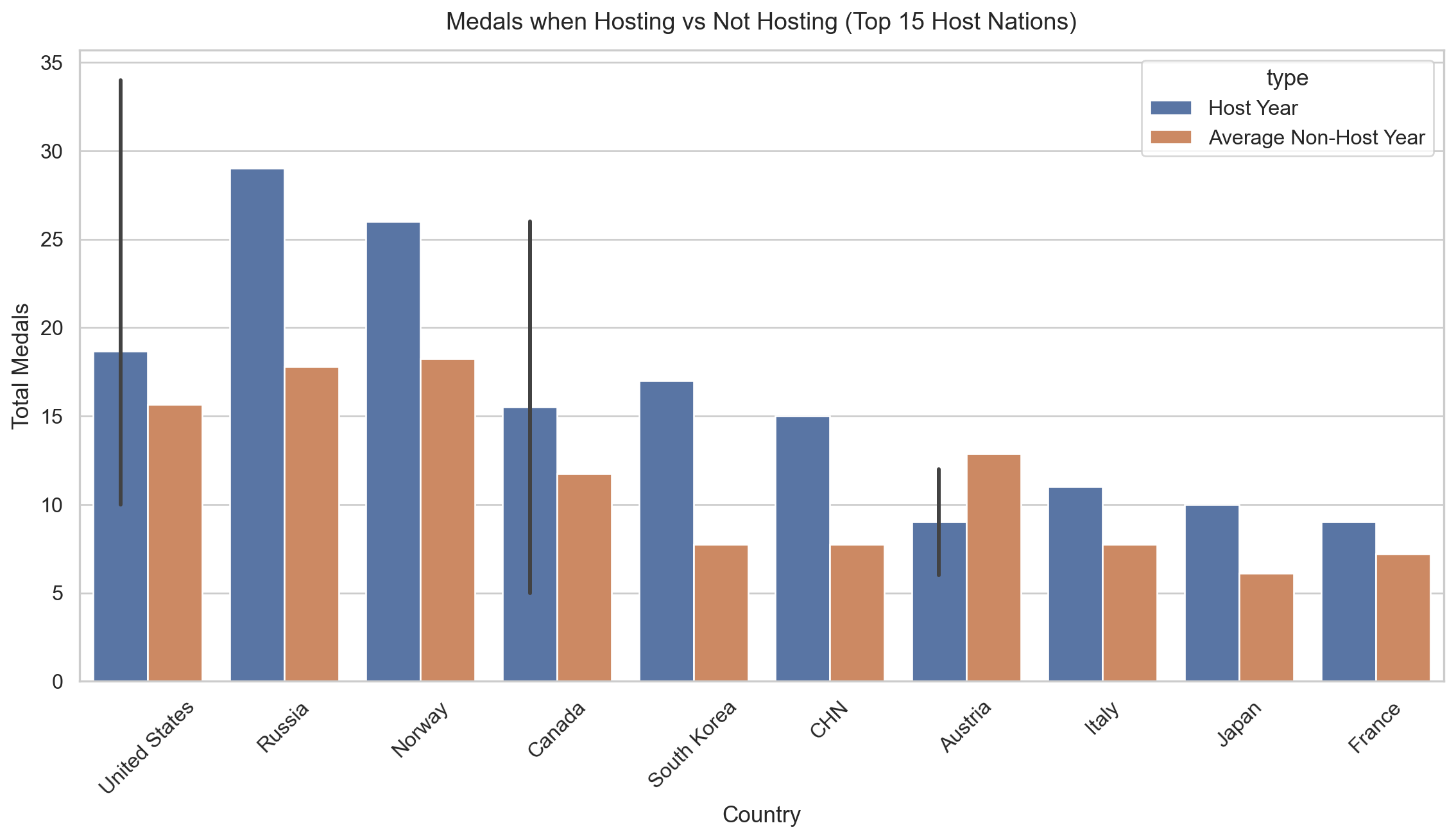
To look at home advantage more directly, I compared each host nations medal count in the year they hosted against their average in all other Games, keeping the 15 nations that won the most medals whilst hosting.

Show code

hosts = (cy[cy['is_host'] == 1][['noc', 'year', 'total_medals']].rename(columns={'total_medals': 'host_medals'}))
non_host_avg = (cy[cy['is_host'] == 0].groupby('noc')['total_medals'].mean().reset_index().rename(columns={'total_medals': 'avg_non_host'}))
compare = (pd.merge(hosts, non_host_avg, on='noc', how='inner').sort_values('host_medals', ascending=False).head(15))
long = compare.melt(id_vars=['noc'],value_vars=['host_medals', 'avg_non_host'], var_name='type', value_name='medals')
long['type'] = long['type'].map({'host_medals':  'Host Year','avg_non_host': 'Average Non-Host Year'})
long['country'] = long['noc'].map(NOC_NAMES).fillna(long['noc'])
fig, ax = plt.subplots(figsize=(12, 7))
sns.barplot(data=long, x='country', y='medals', hue='type', ax=ax)

ax.set_title('Medals when Hosting vs Not Hosting (Top 15 Host Nations)',fontsize=14, pad=12)
ax.set_xlabel('Country')
ax.set_ylabel('Total Medals')
ax.tick_params(axis='x', rotation=45)
fig.tight_layout()
plt.show()

Figure 4: Figure 4: Medal counts in host years versus average non-host performance for the 15 most successful host nations. Most sit noticeably higher in their host year, for example the USA in 2002 (34 medals) and Norway in 1994 (26 medals).

One thing to note is the chart orders by how many medals they won while hosting not by the size of the boost, so the nations on the left aren’t necessarily the ones who benefitted most.

Home advantage is a one time boost. It cannot explain the collapse of nations like the Soviet Union and East Germany, for that political and historical context matters.

6. The fallen powers

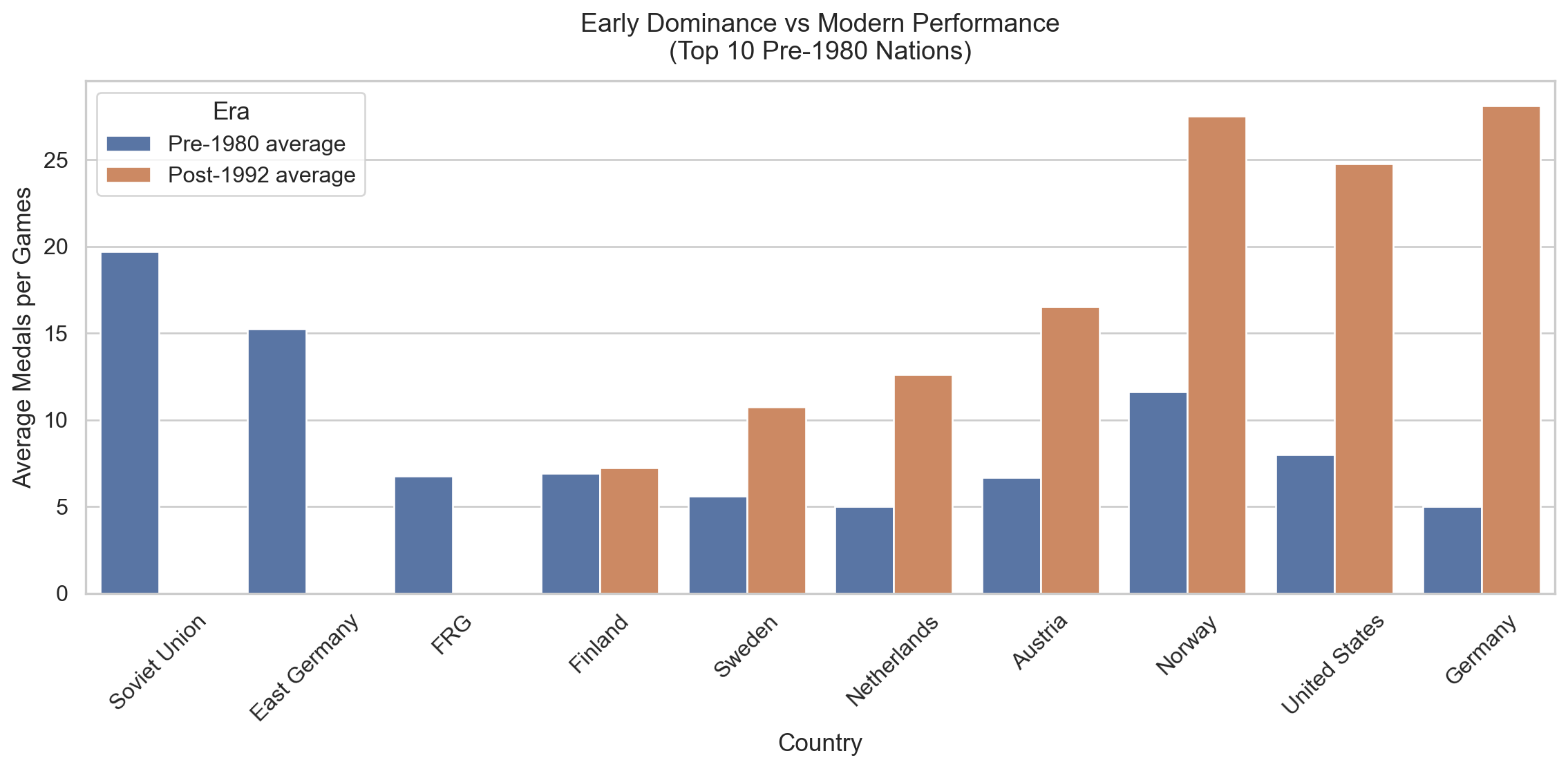
Not every nation that dominated the early era has kept that up. The chart compares the average medals per Games for the top 10 early-era nations looking at results up to and including the 1980 verus their average since 1994. Countries are sorted left to right by the size of their drop off.

Show code

cy_all = final.groupby(['year', 'noc'], as_index=False).agg(total_medals=('noc', 'count'))

early = cy_all[cy_all['year'] <= 1980]
modern = cy_all[cy_all['year'] >= 1994]
early_avg = early.groupby('noc')['total_medals'].mean().rename('early_avg').reset_index()
modern_avg = modern.groupby('noc')['total_medals'].mean().rename('modern_avg').reset_index()

top_early = early_avg.nlargest(10, 'early_avg')['noc']
compare = pd.merge(early_avg[early_avg['noc'].isin(top_early)], modern_avg, on='noc', how='left').fillna(0)
compare['decline'] = compare['early_avg'] - compare['modern_avg']
compare = compare.sort_values('decline', ascending=False)

long = compare.melt(id_vars=['noc'], value_vars=['early_avg', 'modern_avg'], var_name='era', value_name='avg_medals')
long['era'] = long['era'].map({'early_avg': 'Pre-1980 average', 'modern_avg': 'Post-1992 average'})
long['country'] = long['noc'].map(NOC_NAMES).fillna(long['noc'])

fig, ax = plt.subplots(figsize=(12, 6))
sns.barplot(data=long, x='country', y='avg_medals', hue='era', ax=ax)

ax.set_title('Early Dominance vs Modern Performance\n(Top 10 Pre-1980 Nations)', fontsize=14, pad=12)
ax.set_xlabel('Country')
ax.set_ylabel('Average Medals per Games')
ax.legend(title='Era')
ax.tick_params(axis='x', rotation=45)
fig.tight_layout()
plt.show()

Figure 5: Figure 5: Average medals per Games for the top 10 pre-1980 nations, comparing their early era performance against the modern era. The collapse of URS and GDR after the Cold War is the most striking feature.

The Soviet Union and East Germnay show the sharpest drops, likely reflecting the collapse of state-funded sports programmes after the Cold War, which is something a GDP regression cannot capture. Norway and the US have held their ground or improved.

7. The full picture: regression results

7.1 The model

With the data aggregated to country-year level, an OLS regression was run to directly answer the research question: after controlling for GDP per capita and population size, does hosting the Games have a significant impact on medal success? The model is:

Total Medals = β₀ + β₁(is_host) + β₂(log GDP per capita) + β₃(log population) + ε

Show code

import statsmodels.formula.api as smf
reg_data = (pd.read_csv('../data/clean/medals_country_year.csv'))
results_df = (pd.read_csv('../outputs/regression_results.csv'))
print(f"Rows in regression dataset: {len(reg_data)}")
print(f"Countries represented: {reg_data['noc'].nunique()}")
print(f"Host-country observations: {reg_data['is_host'].sum()}")
print()
print(results_df.to_string(index=False))

model = smf.ols('total_medals ~ is_host + log_gdp_per_capita + log_population', data=reg_data).fit()
print(model.summary())

Rows in regression dataset: 332
Countries represented: 42
Host-country observations: 16

          variable      Coef.  Std.Err.         t        P>|t|     [0.025     0.975]
         Intercept -40.866057  5.524349 -7.397443 1.171844e-12 -51.733683 -29.998431
           is_host   4.618627  1.889718  2.444083 1.504838e-02   0.901131   8.336123
log_gdp_per_capita   2.663723  0.332520  8.010721 2.011258e-14   2.009583   3.317864
    log_population   1.433589  0.243437  5.888950 9.621035e-09   0.954694   1.912484
                            OLS Regression Results                            
==============================================================================
Dep. Variable:           total_medals   R-squared:                       0.230
Model:                            OLS   Adj. R-squared:                  0.223
Method:                 Least Squares   F-statistic:                     32.65
Date:                Mon, 06 Apr 2026   Prob (F-statistic):           1.72e-18
Time:                        20:27:50   Log-Likelihood:                -1128.8
No. Observations:                 332   AIC:                             2266.
Df Residuals:                     328   BIC:                             2281.
Df Model:                           3                                         
Covariance Type:            nonrobust                                         
======================================================================================
                         coef    std err          t      P>|t|      [0.025      0.975]
--------------------------------------------------------------------------------------
Intercept            -40.8661      5.524     -7.397      0.000     -51.734     -29.998
is_host                4.6186      1.890      2.444      0.015       0.901       8.336
log_gdp_per_capita     2.6637      0.333      8.011      0.000       2.010       3.318
log_population         1.4336      0.243      5.889      0.000       0.955       1.912
==============================================================================
Omnibus:                       48.817   Durbin-Watson:                   0.779
Prob(Omnibus):                  0.000   Jarque-Bera (JB):               66.730
Skew:                           1.003   Prob(JB):                     3.23e-15
Kurtosis:                       3.895   Cond. No.                         269.
==============================================================================

Notes:
[1] Standard Errors assume that the covariance matrix of the errors is correctly specified.

Show code

comparison = pd.read_csv('../outputs/model_comparison.csv')
comparison.style.set_caption('Table 2: Basic OLS vs Country Fixed Effects')

Table 2: Table 2: Basic OLS vs country fixed effects with only key coefficients

(a) Table 2: Basic OLS vs Country Fixed Effects

	variable	OLS_coef	OLS_pval	FE_coef	FE_pval	OLS_stars	FE_stars
0	is_host	4.619000	0.015000	3.985000	0.001000	*	**
1	log_gdp_per_capita	2.664000	0.000000	1.015000	0.007000	***	**
2	log_population	1.434000	0.000000	26.724000	0.000000	***	***

The basic OLS shows the raw associations between each predictor and medal counts. The fixed effects version asks a harder question, not “whether host countries win more overall” but “whether a country wins more than it normally would when hosting”.

The is_host coefficient drops from 4.6 in the basic OLS to 4.0 in the fixed effects model, a small decrease, but importantly it remains positive and significant ( p = 0.001, stronger than the basic OLS p = 0.015). Strong countries tend to host, so you would expect them to do well regardless, but the advantage survives even when comparing a country against its own baseline.

The log_gdp_per_capita coefficient drops, from 2.664 to 1.015, which makes sense as once I control for country-specific differences, a lot of the gap in wealth between countries is already absorbed. The log_population coefficient in the fixed effects model is unusually large and should be interpreted with caution, as population doesn’t change much within a country over time, so the model doesn’t have much variation to work with. The basic OLS estimate of 1.434 is the more reliable figure for population in this case.

What fixed effects adds

The basic OLS is_host coefficient of 4.6 compares the host country-years against all other country-years. Whereas the fixed effects estimate of 4.0 ( p = 0.001) compares a country against its own historical performance, which is a stricter test that hosting effect passes.

Hosting advantage is real

The basic OLS model estimates that host nations win on average 4.6 more medals than expected after controlling for wealth and population(p = 0.015). The country fixed effects model puts this at 4.0 extra medals ( p = 0.001), which is a smaller but more credible estimate, as it compares each nation against its own baseline rather than against all other countries.

7.2 What the coefficients show

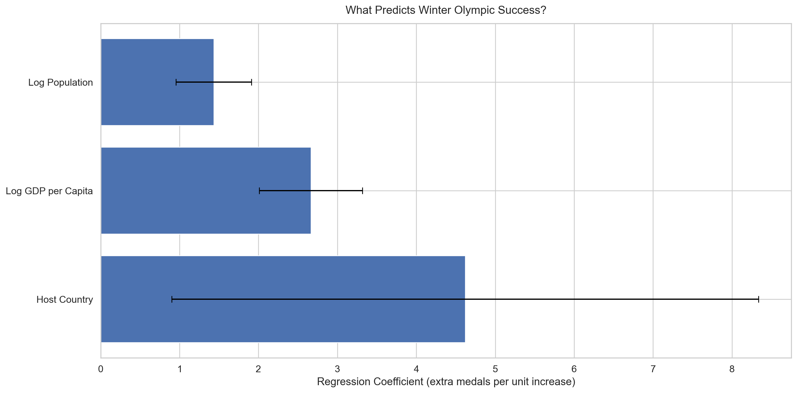
The coefficient plot below pulls together all three results in one view. All three bars fall to the right of zero, meaning hosting, wealth and population all increase expected medal counts. The host status bar looks the longest, but section 8 explains why that is slightly misleading.

Show code

key_vars = ['is_host', 'log_gdp_per_capita', 'log_population']
reg_plot = reg[reg['variable'].isin(key_vars)].copy()
reg_plot['variable'] = reg_plot['variable'].map({'is_host': 'Host Country', 'log_gdp_per_capita': 'Log GDP per Capita', 'log_population': 'Log Population'})
fig, ax = plt.subplots(figsize=(14, 7))
ax.barh(reg_plot['variable'], reg_plot['Coef.'])
ax.errorbar(reg_plot['Coef.'], reg_plot['variable'], xerr=[
        reg_plot['Coef.'] - reg_plot['[0.025'],
        reg_plot['0.975]'] - reg_plot['Coef.']],fmt='none',color='black',capsize=4)

ax.axvline(0, color='black', linewidth=0.8)
ax.set_title("What Predicts Winter Olympic Success?", fontsize=14, pad=12)
ax.set_xlabel("Regression Coefficient (extra medals per unit increase)")
fig.tight_layout()
plt.show()

Figure 6: Figure 6: OLS regression coefficients for the three predictors of Winter Olympic medal success. All bars fall to the right of zero, confirming each factor has a positive impact on medal counts. The error bars show the uncertainty around each estimate, and GDP per capita stands out as the most consistent and reliable predictor due to it having the tightest interval.

The black error bars show the 95% confidence intervals. GDP per capita has the tightest interval of the three, indicating it is the most reliably estimated of the three. The host status bar is wider, reflecting the smaller number of hosting observations in the data.

8. Conclusions

Norway’s GDP per capita is high but not uniquely so. What the regression cannot capture is a century of winter sports culture and the geography that produces competitive athletes across almost every discipline. The model explains the economic and population factors, but Norway’s outlier status sits above them. All three are statistically significant predictors of medal count.

Host advantage is real but limited

The OLS model estimates a boost of 4.6 medals (p = 0.015), tightening to 4.0 under fixed effects ( p = 0.001). The fixed effects result is slightly smaller but more credible, it compares each country against its own baseline rather than against all other nations. The boost is real, but since a country only hosts once every few decades, it explains very little of the long-run medal success. The GDP coefficient falls from 2.664 to 1.015 under fixed effects, as between country wealth differences are absorbed by the country dummies. The population coefficient should be treated with caution in the fixed effects model, as population barely changes within a country over time.

GDP per capita is the strongest overall predictor

From the regression, a 1 unit increase in log GDP per capita is associated with about 2.7 extra medals (p < 0.001), adding up to roughly a 16-medal difference across the full range of countries. Despite the host bar looking longest on the coefficient plot, it only represents a one-time jump, whereas GDP applies continuously across every Games, as well as having more than three times the t-statistic (8.01 vs 2.44) confirming it is the more consistent and reliable predictor across the dataset.

Population matters independently of wealth

Population also plays an important role, even after accounting for wealth. A 1 unit increase in log population leads to about 1.4 additional medals (p < 0.001). Across the full range of countries, this again adds up to roughly a 16 medal difference, which is comparable in scale to the GDP effect.

Bottom line

Three things shape how well a country does at the Winter Olympics: wealth, population, and whether it is hosting. The OLS model estimates a hosting boost of 4.6 medals tightening to 4.0 medals under the stricter fixed effects test. GDP per capita has the most reliable and consistent effect across both models. So if you are trying to predict how many medals a country might win, GDP per capita on its own gets you most of the way there.